Pandas is an incredible data ingestion and processing package. Thanks to it’s simplicity and utility, it has become the de-facto choice in the Data Engineering and Data Science fields.

To get started with Pandas, ensure you have Python installed and have activated your desired environment. If you are unsure what a Python environment is or how to use them, you can quickly get up to speed by reading my article on it:

Python Environments: An Overview

If you haven’t installed Pandas you can by entering the following in your terminal:

pip install pandas

Next I would recommend creating a Juypter Notebook (although you can use a regular python file) by using your text editor to create a file called tutorial.ipynb or by entering the following in your terminal:

touch tutorial.ipynb

Open tutorial.ipynb in your text editor of choice and then import the Pandas library by typing the following:

import pandas as pd

Creating and Saving a Pandas DataFrame

Reading a CSV to a DataFrame

A CSV is a Comma Separated Values file. It can be thought of as a simple table with rows and columns, where each column is separated by a comma and each row by a new line.

If you would like to follow along with this tutorial exactly, I have provided the example dataset I made in the repository below:

Reading a CSV is as simple as the following (assuming example.csv is in the same directory/folder that your Jupyter Notebook is in):

people_df = pd.read_csv("./people.csv")

If you would like to read only certain columns (great for conserving memory if possible), you can instead run:

people_df = pd.read_csv("./people.csv", usecols=["first_name", "last_name"])

Chunking for Large CSVs

As you work on bigger, more complex Data Science projects, you find that your computer doesn’t have enough memory to import a CSV or set of CSVs. Or even more likely, there is not enough memory to perform an operation on one or more CSVs (for example a join on two large dataframes).

One strategy Data Scientists use is to “chunk” the CSV out, which essentially means to read the CSV piece by piece. For example, the following code loads 100 rows into the chunked_df dataframe, which is a dataframe created on each iteration of the for loop until the entire CSV has been read:

mean_chunk_ages = []

for people_chunk_df in pd.read_csv("./people.csv", chunksize=100):
    mean_chunk_ages.append(people_chunk_df["age:int"].mean())

print("Average age for each chunk:", mean_chunk_ages)

Creating a DataFrame using Data Structures

There may be times where instead of creating a dataframe by reading a file, you would like to create it from a data structure you have in Python. The two main ways of doing so are by using lists and dictionaries as shown below.

Creating a DataFrame from a List

list_df = pd.DataFrame([[1, 2, 3], [4, 5, 6], [7, 8, 9]], columns=["a", "b", "c"])
list_df # typing a variable name in a cell will display it's contents if in a Jupyter notebook

Creating a DataFrame from a Dictionary

dict_df = pd.DataFrame({"a": [1, 2, 3], "b": [4, 5, 6], "c": [7, 8, 9]})
dict_df # typing a variable name in a cell will display it's contents if in a Jupyter notebook

Displaying a DataFrame

As shown in the previous section, you can display the contents of a dataframe simply by typing it’s variable name in a cell within a Jupyter Notebook. This was demonstrated with the list_df and dict_df dataframes.

However, there may be times when you wish to display a smaller portion or specific slice of a dataframe. This can been done using the methods outlined below.

Head and Tail Methods

The head() method displays the first five rows of a given dataframe:

people_df.head()

The opposite of head() is also available via the tail() method, which returns the last five rows of a given dataframe:

people_df.tail()

List Slicing

List slicing is a syntax that Python provides out of the box, to return a certain contiguous portion of a list:

nums = [4, 5, 6, 7, 8]
print(nums[1:4]) # prints: [5, 6, 7]

List slicing can also be applied to dataframes:

people_df[10:20] # will display rows 10 to 19

Combining DataFrame Together

Pandas provides methods to help you combine two or more dataframes together. However, to properly utilise these methods it is important to understand how the joins work.

I recommend this article if you would like to learn about joins in more depth: Image from: Joins in Pandas

However, as a quick refresher, these are the five types of joins available in pandas:

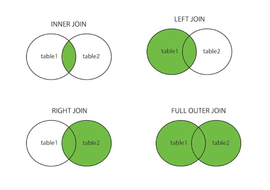
Image from: Joins in Pandas

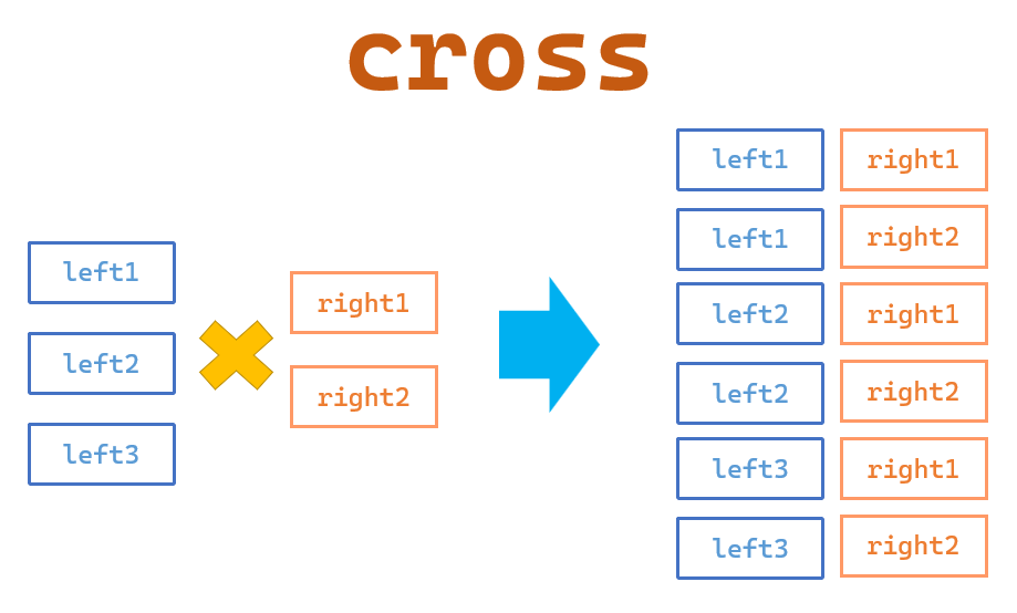
Image from: Pandas >> Data Combination(1): merge()

Combine DataFrames using Merge

The merge() method can be used to join two dataframes together. In the following example, two dataframes are created; people1_df and people2_df.

people1_df = people_df[["first_name", "last_name", "genre"]][:500] # first 500 people
people2_df = people_df[["first_name", "last_name", "genre"]][500:] # last 500 people

Then an inner join is used to return only people who have the same favourite genre:

people1_df.merge(people2_df, how="inner", left_on="genre", right_on="genre")

Conditional Filtering

Filtering a dataframe to find certain values or rows is a very common use case when using Pandas. There are multiple approaches to doing so but the simplest is to just use a conditional statement as shown below:

# displays all people with a bot score between 0.5 and 0.75
people_df[(people_df["bot_score"] >= 0.5) & (people_df["bot_score"] <= 0.75)]
# displays all people with the first name Mark
people_df[people_df["first_name"] == "Mark"]
# displays all people with the first name Mark or John
people_df[people_df["first_name"].isin(["Mark", "John"])]
# displays all people who don't have the name Mark or John
# the not condition is done using the ~ symbol
people_df[~people_df["first_name"].isin(["Mark", "John"])]

Looping over a DataFrame

genre_freq_above_age_50 = {}

for i, row in people_df.iterrows():
    if row["age:int"] > 50:
        genre = row["genre"]

        if genre not in genre_freq_above_age_50:
            genre_freq_above_age_50[genre] = 0

        genre_freq_above_age_50[genre] += 1

print(genre_freq_above_age_50)

Field Manipulation

Adding a Field

If you have a list have is the same length of your dataframe you can add it by assigning it to a new key/field (similar to dictionaries). For example, random_numbers is a list of 1000 random numbers and the people_df also has 1000 rows. As such if we wanted to add this such that row n in people_df has the random number of random_numbers[n], you could do the following:

random_numbers = [random.randint(0, 20) for _ in range(1000)]
people_df["random_number"] = random_numbers

If you wished to assign a singular value to all rows of the people_df you can use the same syntax but with a single value instead of a list:

people_df["greeting"] = "Hello! How are you?"
people_df["num_warnings"] = 0

Deleting a Field

Deleting field(s) is simple using the drop() method:

people_df.drop("random_number", axis=1, inplace=True) # delete a single field
# delete two fields using a list
people_df.drop([":LABEL", "random_number"], axis=1, inplace=True)

Renaming a Field

Renaming fields is done using the rename() method which uses the key to identify the original name of the field and the value to specify what you would like to rename the field to.

In the following example I rename the birth_date:date and bot_score:float fields to birth_date and bot_score.

people_df.rename({ "birth_date:date": "birth_date", "bot_score:float": "bot_score" }, axis=1, inplace=True)

Modifying the Values of a Field

You can modify each value in a field by defining a function that converts the input value from the dataframe, into a the desired output and passing that function to the apply() method.

In the example below, I wrote a function which capitalises each word in the genre field unless the word was “and”.

def capitalize_words(text):
    words = []

    for word in text.split(" "):
        if word != "and":
            words.append(word.capitalize())
        else:
            words.append(word)

    return " ".join(words)

people_df["genre"] = people_df["genre"].apply(capitalize_words)

# one of the original values from genre: "Business and entrepreneurship"
# updated value: "Business and Entrepreneurship"

The apply() can also be used to create a new field from an existing field, simply by using a key that doesn’t exist in the original dataframe. For example:

people_df["updated_genre_name"] = people_df["genre"].apply(capitalize_words)

Removing Duplicates

The drop_duplicates method can be used to remove duplicates from a dataframe. The subset argument is used to define what set of field values need to be duplicated, to be considered a duplicate.

In the following example, only the personId:ID(Person-ID) needs to be the same to be considered a duplicate.

existing_person = people_df.iloc[0].tolist()
# add a person who already exists in the dataframe three times
# at the bottom of the datafram
people_df.loc[len(people_df)] = existing_person
people_df.loc[len(people_df)] = existing_person
people_df.loc[len(people_df)] = existing_person

print(len(people_df)) # 1003
people_df.drop_duplicates(subset=["personId:ID(Person-ID)"], inplace=True)
print(len(people_df)) # 1000

Saving a DataFrame to a CSV

Finally, the last task you may like to conduct is saving your newly processed dataframe to a CSV. This can be done using the to_csv() method:

people_df.to_csv("./updated_people.csv", index=False)

As shown above, I would also suggest setting index to False as in most cases you don’t want your rows numbered.

Conclusion

In conclusion, the Pandas library is a crucial tool for anyone working with data in Python. Its wide range of functionalities allows you to easily manipulate and analyze data - from reading and writing files, creating and modifying dataframes, to conducting in-depth analysis with filtering and merging. The ease with which you can perform these tasks makes Pandas a versatile and powerful tool in any data scientist’s toolkit. With the basic understanding and skills acquired in this tutorial, you’re now ready to dive into your own data science projects using Pandas.

If I forgot any useful methods or properties you use on a regular basis, please comment below and I may add them to the article or in a new post!